Each day, Picnic delivers groceries to tens of thousands of customers. To do this as efficiently as possible, operations follow a plan created the day before the actual deliveries. This so-called Master Planning Process (MPP) represents the planning of the Picnic supply chain path for every ordered article from the Fulfilment Centre to the customer’s door.

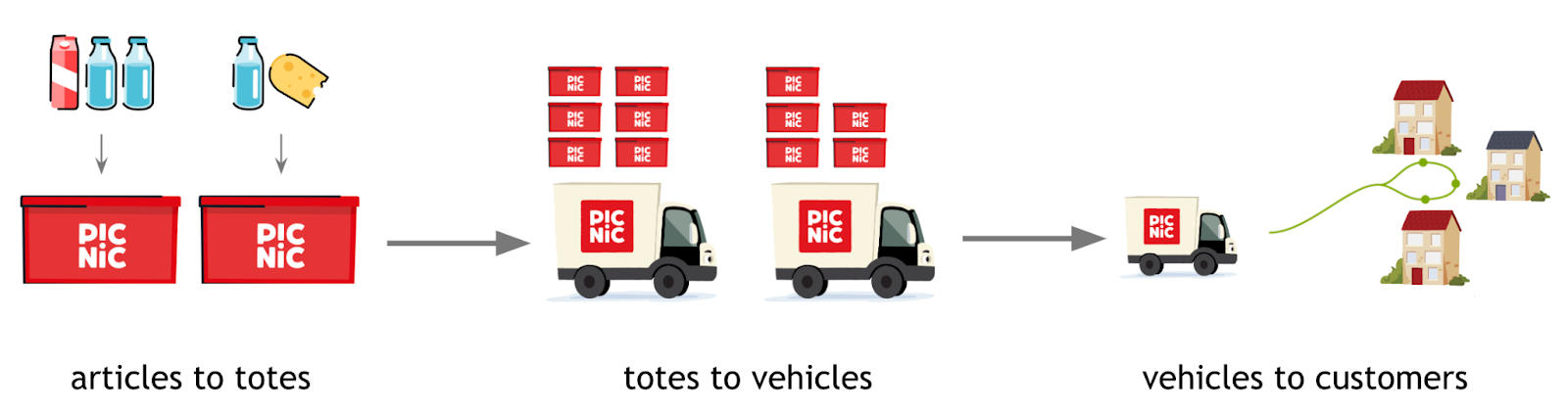
As the scale of operations is quite large, Picnic uses various algorithms for each stage of the MPP to automatically generate a planning. These plans must not only be feasible, but also ensure a high quality of service for the customers. For example, when assigning articles to totes, the goal is to distribute the articles in a way that minimises the number of totes needed. However, the fragility of articles is also taken into account such that fragile articles (e.g. fruit) are preferably not placed next to bulky articles (e.g. large bottles of coke).

For us humans, it’s relatively easy to come up with a good plan. When packing a bag ourselves, most of us will intuitively put the fragile articles on top. Also, when travelling to a location, we often choose the most direct route possible. Computers lack this sense of intuition — a plan needs to be generated and evaluated mathematically to determine its effectiveness. But how exactly are these plans created, and how can they be assessed?

To answer these questions, we’ll dive into the field of combinatorial optimisation. If you have never heard of this before, don’t worry. A short introduction to this field is given below. After this introduction we’ll discuss TimeFold, which is an open-source solver that Picnic uses to find solutions for combinatorial problems.

What is combinatorial optimisation?

Combinatorial optimisation is the process of trying to find the optimal solution given a set of finite possibilities. As the name suggests, the optimal solution is represented by a combination or arrangement of the provided variables that need to be planned. A solution is optimal if it minimises or maximises an objective function, while adhering to the provided constraints.

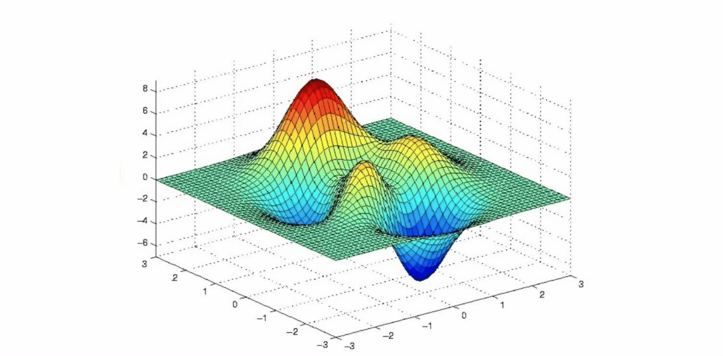
An objective can be any goal, such as the minimisation of the amount of planned vehicles or the maximisation of their stability. An objective function is the mathematical expression of one or more objectives, where each objective is given a certain weight to signify its importance. If we were to plot the objective function of a combinatorial problem, we’d end up with a graph looking as follows:

In this graph, each possible solution is mapped to its corresponding objective score. In case we are trying to maximise the objective function, the indicated global optima represents the best solution(s). Other peaks represent so-called local optima. A local optimum is a solution that is optimal within a neighbouring set of solutions. The tricky part of combinatorial optimisation is discovering which solutions are part of the global optima. To be absolutely sure that a solution leads to the best objective score, one would need to try out every possible solution. This approach, known as exhaustive search, is a form of exact solving. Unfortunately, in many practical cases, trying out every solution is not a viable approach due to time and/or resource constraints.

There are some techniques that can be used to speed up the search. For example, a branch-and-bound algorithm can prune solutions, by deducing that no better score can be achieved in certain areas of the search space. But even with such optimisations, the required computing power to find the best solution(s) is too much for many large problems.

Instead of exact solving, so-called heuristic algorithms can be used to efficiently explore the search space. These algorithms employ various strategies aiming to find good solutions quickly. The downside of using heuristics is that they can’t guarantee that the best solution found is also the most optimal. Luckily, in a lot of cases, optimality is not a necessity. Often there is simply a need for a solution that is ‘good enough’.

An immense amount of research is done on heuristic algorithms and diving into each algorithm requires more than just one blog. For now, all that is needed to be known is that heuristics commonly explore the search space by keeping track of various solutions. They iteratively adjust a solution in the hope of achieving better results over time. As heuristics don’t know when an optimal solution is found, they simply return their best found solution after some criteria is met. Such a criteria can, for example, be a time limit or a minimum/maximum value for the objective score.

One of the simplest heuristics is called Hill-Climbing. As the name suggests this heuristic will explore the search space by only accepting solutions that improve the objective score. However, as can be seen in the animation below, hill-climbing tends to get stuck in local optima as it can not find better solutions in its search neighbourhood.

There are many ways to circumvent this. One simple and popular approach is called Late Acceptance Hill-Climbing. This approach accepts solutions if they are at least as good as the best found solution x steps ago. Because of this, the algorithm is able to accept worse solutions, which allow it to escape a local optimum. However, it does come at a performance cost as it needs to maintain a history of solutions, requiring additional memory operations and comparisons.

Many more heuristics exist, each with their own advantages and drawbacks. Choosing which one fits your use case the best could simply be a matter of trying them out and comparing their performance. At Picnic, we prefer to build most of our software in-house, but that doesn’t mean we need to reinvent the wheel every time. Instead of implementing each heuristic ourselves we can use one of the many open-source solvers that implement various exact algorithms and heuristics. One such solver is TimeFold, which Picnic has been using for key components of the MPP for the past year.

TimeFold

TimeFold is a relatively new solver and has been forked from OptaPlanner by its original creator. Compared to its predecessor, it has made various improvements under the hood that enable it to perform at twice the speed.

Why TimeFold?

After some internal testing, TimeFold was chosen as the best fitting solver for Picnic’s use case. It was benchmarked against other popular Java solvers, including Google-OR Tools and Choco solver. For each solver, a small proof of concept (POC) was made. Every POC shared the same objectives and constraints, and was tested on identical datasets. Comparisons were based on the following aspects:

• Solution quality: How good are the solutions?
• Runtime: How much computation time is needed?
• Maintainability: How easy is the code to understand and extend?
• Scalability: How well does it scale to larger instances?
• Documentation: How good is the online documentation?

Each solver achieved similar results in roughly the same time for small to medium instance sizes. The level of documentation was also great for all of them. However, only TimeFold was able to scale well to instance sizes that were required for the Picnic use case. This was somewhat expected, as only TimeFold is advertised to be tuned towards solving large problems well in a relatively short timespan.

Another great advantage of TimeFold is its excellent maintainability. It allows constraints and objectives to be defined through a stream-like API, which makes it relatively trivial to add new requirements. For other solvers, it is much harder to do so since their constraints and objectives are defined in a more mathematical manner. An example of TimeFold’s stream-like API is given below, defining a constraint that limits the total volume of articles in a tote.

Constraint toteVolume(ConstraintFactory constraintFactory) {
        int maxToteVolume = 100;

        return constraintFactory
                .forEach(Article.class)
                .groupBy(Article::getTote, sum(Article::getVolume))
                .filter((tote, volume) -> volume > maxToteVolume)
                .penalize(HardSoftScore.ONE_HARD)
                .asConstraint("Tote can't exceed maximum volume");
    }

In the code above, TimeFold groups each article by their tote and filters on totes that have their volume above a certain threshold. Every tote that passes this filter is then penalised as a constraint violation.

Structure

TimeFold processes the constraints and objectives that are programmatically provided by mapping the constraints to a HardScore and the objectives to a SoftScore. The HardScore represents the total number of violations across all constraints, while the SoftScore indicates the cumulative value of how well each objective has been met. Each constraint and objective can also be given a weight. For example, if in the constraint above three totes are over their volume limit, the solution would have a HardScore of -3. If this constraint would be given a weight of 3, the HardScore would be -3 * 3 = -9. At Picnic all constraints have the same weight, as any violation is already unacceptable. However, weights of objectives are tuneable, which allows the planning to be very flexible to the needs of the business. If one day it is decided that we want to put more emphasis on quality of service compared to efficiency (or vice versa), we can simply raise the weights of the relevant objectives.

In order to start solving, TimeFold first creates something called a problem. A problem contains the following properties:

This problem is passed along to a solver, together with the objectives, constraints and configured search algorithm. The solver returns the best solution it can find for the problem by allocating its planning entities and adhering to the problem facts.

To find good solutions, a problem is solved in two phases. First a construction heuristic is started, which quickly generates a (near) feasible solution. Afterwards, the search phase tries to improve the initial solution by iteratively adjusting previously created solutions.

Construction Heuristic

The construction heuristic creates an initial solution in a greedy manner. That means that for every planning entity it assigns, it will always choose the assignment that is optimal at that moment. An approach that has been proven to work well for placing articles to totes, is to start with the items that have the largest volumes and to place them into the first tote that fits them. This is also called first-fit-decreasing.

The construction heuristic only cares about achieving a feasible solution, so there is no need to evaluate the objectives. Combining this with the fact that the construction heuristic is a greedy algorithm, makes it much faster than the search phase.

TimeFold supports over 10 types of construction heuristics out of the box, including first-fit-decreasing. These construction heuristics can also be further tweaked, as we at Picnic have done as well. For example, our insertion order is not based only by volume, but also by weight, fragility and other factors.

Search Phase

As mentioned before, the search phase iteratively adjusts solutions to explore the search space. TimeFold supports 8 different local search algorithms, such as Late Acceptance Hill-Climbing. There is also promised support for genetic algorithms in the future. If you are interested in reading about genetic algorithms, there is another Picnic blog written about this topic here.

To adjust solutions, TimeFold uses so-called moves. The following moves are implemented by TimeFold out of the box:

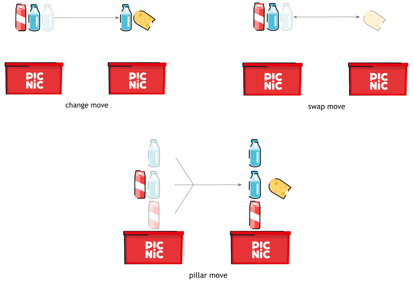
TimeFold also allows for any user defined custom move. For example, one can define a move that guarantees that a swap only occurs for articles of the same fragility.

Another handy feature of TimeFold is move filtering. When a move is suggested, one can define certain filters that prevent it from being evaluated. This can be useful if the calculation of the problem score is computationally intensive, which is the case for the Picnic use case. Some of our algorithms have more than forty constraints and objectives. Thus, if we can prevent a portion of moves from being evaluated, we save a lot of wasted computation time.

So which moves can be filtered out? This is problem specific, but moves are generally filtered out if they are guaranteed to lead to infeasible solutions or don’t change the state of the solution. A simple example is the swapping of two identical articles. We know that performing this move will not change the state of the solution, so evaluating it will never be beneficial. Another example is the separation of temperature zones. Picnic offers ambient and cooled products. Each vehicle has one frame for ambient and one frame for cooled articles. Thus, if a move suggests to place an ambient tote in a cooled frame, we know it will never lead to a feasible solution and can thus be filtered out.

It should be noted that move filtering can also reduce the performance of the algorithm. Each move must first pass this filter, which requires computation time. Thus, if the amount of moves that can be filtered is small or if the filter calculation is complex, it might be better to simply evaluate the HardSoft score of every move.

Benchmarking

TimeFold has a built-in benchmarker, which can be used to see how the solver finds solutions over time. This is extremely useful for determining its performance and has been vital to the success of its integration with the MPP. With the benchmarker, various search algorithms can be applied on provided problems. After which their solution quality over time can be compared.

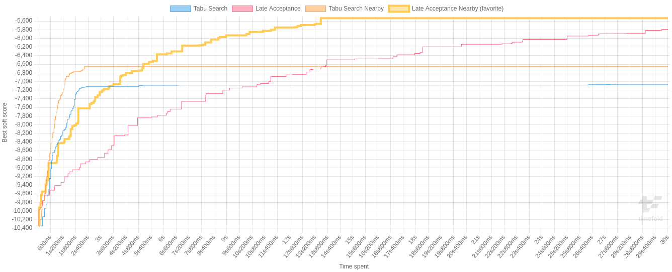
These graphs can aid us in deciding which search algorithm to choose. For example, if we are time constrained, Tabu Search Nearby could be the best choice for the problem provided above, as it generates good solutions the fastest. However, Late Acceptance Nearby might be a better fit if computation time is less of a concern, since it achieves better results in the end.

As these conclusions are drawn from a single graph (i.e. one problem instance), they can’t guarantee the same performance for different inputs. Thus, one should run each search algorithm on various datasets to see if there is a general pattern.

Not only does the benchmarker tell you which search algorithms perform the best. It can also give an indication on how well a specific algorithm explores the search space. By observing the shape of the solution quality over time, some conclusions can be drawn.

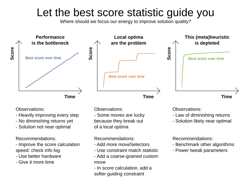
When using TimeFold it is highly recommended to follow the guide above, as acting on the provided observations can significantly improve the computation speed and solution quality of your algorithm.

Summary

Solving combinatorial problems is at the core of Picnic’s tech identity. Doing this well allows us to efficiently deliver groceries to customers, while adhering to a high quality of service. We are planning articles to totes, and totes to vehicles by using an open-source solver called TimeFold. This solver allows us to easily set up business objectives and constraints, and quickly adjust requirements when needed. Many of TimeFold’s features, such as move filtering and benchmarking, are used to improve our algorithms and get better results in a shorter timespan. By not trying out every solution, but instead smartly navigating the search space, we can generate good results in a relatively short amount of time. Not only does this allow us to serve many customers today, but it will also support us in our future growth.