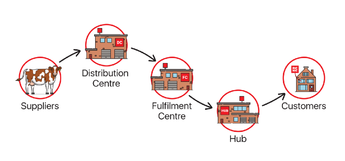
What do designing an aircraft wing, packing boxes into a container and making timetables have in common? They’re all optimization problems. There’s an objective to be maximized or minimized (least air resistance, most boxes packed or least man hours spent). Each individual solution to these problems will have a score for the objective and the goal is to find the best possible one. In a previous blog post we discussed how the world of logistics is fundamentally one of algorithms and optimization. In this blog post we’ll zoom into one specific case. Each day tens of thousands of orders for Picnic’s customers are packed at our warehouses (or fulfilment centers as we like to call them). These orders are loaded into trucks and shipped to our hubs, from which they are delivered to the customer’s doorstep. How do we create an optimal schedule for these trucks driving between fulfilment centers and hubs?

Genetic Algorithms: Digital Evolution

At Picnic we use a Genetic Algorithm (or GA for short) to solve this truck scheduling problem. GAs are a great tool to solve problems when it is impossible to consider every possible solution because there are simply too many. Instead GAs consider only a fraction of the solutions. This is achieved by taking inspiration from Darwin’s evolutionary theory: letting a population of individual solutions reproduce while subjecting them to natural selection gradually improves the whole population. This is done until the population contains a solution that is deemed “good enough”.

Let’s consider a game, a greatly simplified version of Lingo, and design a GA to play the game. In this game a word of known length (e.g. the 6 letter word “picnic”) has to be guessed. When the GA submits a guess, the game will respond with the number of letters that are correct (the right letter at the right location). For example, when the GA guesses “pifnit”, the game’s response will be 4. For this game, the GA will get an unlimited number of guesses.

Step 1: DNA

In a GA each individual in the population represents a possible solution. Each individual has DNA, often represented as a sequence of numbers or characters. Usually, a big challenge in implementing a GA is to fit a solution within this format. Luckily, in this case modeling the DNA is trivial: since we’re looking for a string, the DNA is simply a sequence of characters.

Step 2: Initial Population

The first step of running the GA is to generate the initial population. Usually, this is achieved by simply generating random DNA sequences. For our game, we’ll start with the following initial population: “ugjhel”, “prjuyj”, “gbenih”, “bxoagp”, “yiptor” and “zyglcs”.

Step 3: Natural Selection

Each generation of individuals will face the GA equivalent of natural selection: the best solutions will be allowed to reproduce while the rest will be forgotten. We want to maintain diversity in our gene pool. This prevents us from getting stuck with a population of good individuals, but with only limited potential to produce the best individual. We’ll apply a method called Tournament Selection to achieve this, but many other methods exist.

During tournament selection we’ll divide our population into groups randomly (the tournaments) and pick the best individual (having the most correct letters) from each one. For example we could divide the population generated in step 2 into two tournaments: “ugjhel”, “prjuyj” and “bxoagp” are a single tournament. “gbenih”, “yiptor” and “zyglcs” make up the other. The winner of the first tournament is “prjuyj” (1 correct letter). “gbenih” (2 correct letters) wins the other. They will move on to the next phase: reproduction.

Step 4: Reproduction

After individuals with a low fitness have been eliminated, the remaining ones will reproduce until the population reaches its original size. When reproducing, the DNA of two individuals is combined. We split both individuals’ DNA at (the same) random point, pasting two parts together and discarding the others. This process is called crossover. After crossover, there’s a random chance that each character in the new individual’s genome will be changed to another random one: mutation.

Both crossover and mutation mimic their natural counterparts. Together they ensure that there is enough variation in the gene pool, while moving closer to an optimal solution with each generation.

Our parents “prjuyj” and “gbenih” will produce 4 children (for example “prenih”, “prguyj”, “geeuyj”, “prjuyh”) to reach the original population size of 6 individuals. Out of this offspring, “prenih” has actually improved on its parents since it has 1 additional correct letter.

After refilling the population, the GA moves back to step 3. It continues this cycle of reproduction and natural selection until its population contains an individual that has 100% correct characters. One particular run of this algorithm is graphed below, showing the quality of the best individual in each generation and the average of all individuals. Its population contained “picnic” after 36 generations, meaning it had to guess the word 216 times (evaluating every individual for every iteration). This is a huge improvement over searching all 308,915,776 possibilities.

Truck Scheduling Algorithm

After playing our very simple word guessing game, we can conclude a few things about GAs:

• They generate many different solutions to a problem, getting progressively better, but without having to explore every single solution.
• Each of the generated individuals has to be evaluated.
• They have a number of mechanisms to prevent getting stuck at suboptimal solutions.

Before our word guessing game we mentioned Picnic uses a GA to solve the problem of scheduling trucks. So how do we implement this, more complex, problem as a GA and how does it perform?

Before making the truck schedule, our algorithms have already determined which groceries should be packed together in a shipment (a truck trailer full of groceries). The input to the GA are these shipments, which need to go from a warehouse to a hub before a certain time. Additionally we’ve estimated the number of trucks we will require and input that to the GA too. The GA will then calculate which truck takes which shipment at what time. As the number of shipments and trucks grows, the number of possible shipment-to-truck mappings explodes. This indicates that a GA is a good fit for this problem, since we cannot try out every possible option.

Modeling

Usually, the biggest challenge in implementing a GA is modelling the DNA. We have to make sure that the DNA supports crossover and mutation, while keeping it easy to evaluate the quality of an individual.

In our model each truck and shipment is assigned an incrementing integer ID. For example, if on a given day 2 trucks will be driving from Picnic warehouses to hubs they will be labelled Truck 0 and Truck 1 for that day. If there are 4 shipments that day, they will be labelled Shipment 0, Shipment 1, Shipment 2, Shipment 3. Given this information, the DNA for the whole truck schedule can just be one big list of integers. In this list each index represents a shipment ID and each value represents the truck ID this shipment will be transported by. There is one catch though, since we want each truck to have at least one shipment. To ensure this we simply assign each truck one initial shipment and do not put these shipments in the DNA. Because of this, the length of each individual’s DNA is equal to: number of shipments — number of trucks.

Now that we have modeled assigning shipments to trucks, we need a way to build a complete schedule. We achieve this simply by looking at the latest departure time of a shipment. We fill up a truck’s schedule from the back to the front, starting with the shipment that can depart the latest and adding shipments until none remain.

So, for example, if we have the following shipments which should fit into 2 trucks:

Then our DNA could look like this: [1, 2]. And the resulting schedule would be the following:

In this case, there’s a gap between Shipment 0 and 2 so Shipment 0 can depart in time. Shipment 3 will depart an hour earlier than its latest departure time to make it fit before Shipment 1.

Since this is a GA we need to evaluate the individuals. In this case we’d like to have as much time as possible to prepare each shipment in the warehouse. So as an objective function we’ll take the sum of differences in shipments’ latest departure time and actual departure time. In the above solution this would be 1 hour and the optimal solution would be 0 hours.

Performance

For the DNA described above, even if there are only 15 shipments and 5 trucks, the number of possible individuals is 9,765,624. The goal for our GA is to find a solution while evaluating significantly fewer individuals.

The graph below shows one run of our GA for 30 shipments and 15 trucks (making the possible number of individuals much higher than the 9,765,624 mentioned above). It shows the sum of deviations from the latest departure time, both for the best individual and the average of each generation’s population. It found an optimal solution in just 14 generations of 100 individuals (so only evaluating 1400). Making it much more efficient than iterating over all solutions.

The disadvantage of all GAs, including this one, is that they might never find the optimal solution. A good strategy is to cut off the GA after a number of generations without improvement. This way you will always end up with a good enough solution in reasonable time.

Conclusion

Genetic Algorithms are a great way to approximate solutions to optimization problems in a reasonable time. At Picnic things move fast. In our truck scheduling problem we introduced way more constraints than described here. For example, we make sure that enough storage space for arriving shipments is available at our hubs. Luckily, these changes are easily made to a GA by just including them in the objective function evaluating individuals. We need to solve these kinds of newly arising problems continuously and update our existing solutions for new situations. GAs are one tool in our toolbox, which we expand and improve on a daily basis.