
Chapter 1: The road to hell is paved with good intentions.
A Simple Question at Scale
At Picnic, delivering groceries isn’t just about moving groceries from A to B — it’s about doing so efficiently, sustainably, and at scale. Every day, hundreds of thousands of orders flow through dozens of hubs. Behind it all lies a deceptively simple question: how many deliveries will each hub handle tomorrow?
The answer drives capacity planning, staffing, routing, and vehicle allocation — and even small forecast errors ripple through the entire chain. Demand shifts with weather, promotions, holidays, and customer behavior, so accuracy is both critical and difficult.
Over the past three years, we’ve worked to strengthen our forecasting system, built around an ML-powered Temporal Fusion Transformer (TFT) that predicts deliveries per hub and daypart 1–14 days ahead using calendar and operational signals. Along the way, we made design choices that solved short-term problems but later became constraints. In particular, the inclusion of a feature in our model, the confirmed deliveries, which gave us amazing short term accuracy, and the expense of reshaping our entire forecasting solution.
In this article, we will tell the story of our journey including this feature in our system and the lessons we learned through it. Please, keep in mind that, with the magic of hindsight, some of the problems with our decisions may seem obvious now, but back then, on the day to day of a fast-paced company experiencing a rapid growth to new markets, our perspective was very different. Enjoy the ride!

Adding complexity: unconstrained demand and intra-day forecast
From a planning perspective, the ideal target to forecast is unconstrained demand — the number of deliveries customers would place if capacity were unlimited. This is the demand that reflects true customer intent and is most useful for long-term capacity planning and strategic decisions. In reality, however, our system is constrained by operational limits. When a hub runs out of capacity, delivery slots are closed and observed demand becomes capped by what we can physically deliver.
As a result, our forecasting problem evolves over time. Far ahead of the delivery date, we want the model to reason about unconstrained demand, the real capacity. But as the delivery date approaches and capacity constraints start to bind, we need to update our forecast to increasingly reflect constrained demand.
In addition, we have a second dimension of complexity. Our operational teams require intra-day updates as orders are placed. During the final hours before cutoff, planners track booking dynamics at an hourly resolution to detect deviations from expected demand curves and rebalance capacity when possible. In particular, the last 48 hours before delivery are the most critical for our forecast.
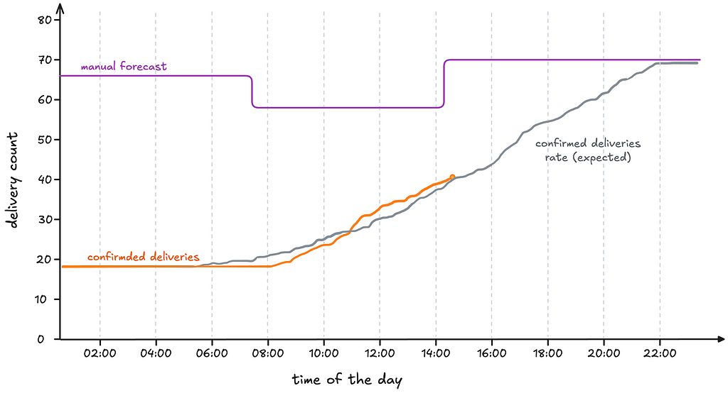
Figure 2 illustrates why intra-day updates are essential. It shows the cumulative number of confirmed deliveries throughout the day for a specific hub, delivery period, and date. As a benchmark, we also plot the confirmed deliveries from three weeks earlier for the same hub and weekday. This historical curve serves as a reference for the expected shape of booking dynamics on a typical day; let’s call this shape the confirmed deliveries rate.
When the current confirmed deliveries begin to deviate from the confirmed deliveries rate, analysts manually adjust the initial forecast upward or downward as it is required. To avoid overwhelming the team, these corrections are performed only twice per day. Our goal was to give the ML model the same ability: to detect deviations in real time and react accordingly.
For us, the time-granularity disparity (days and hours) meant the same forecasting system had to operate across two distinct regimes. At longer horizons, predictions are driven primarily by slow-moving signals such as calendar effects, seasonality, and structural differences between hubs. In contrast, intra-day forecasting emphasizes short-term dynamics: recent booking pace, partial order information, and operational disruptions that only become visible close to delivery. As the delivery date approaches, the problem shifts from estimating aggregate future demand to continuously updating expectations based on partial observations.
Here, we took an important design decision: rather than building two separate models — one optimized for day-ahead planning and another for intra-day updates — we chose to use a single model across both contexts.
This decision was driven by a few practical considerations. First, maintaining one model simplified the operational footprint: fewer pipelines, less duplicated feature engineering, and a smaller surface area for maintenance and monitoring. Second, a unified model ensured consistency between long-term and short-term forecasts, avoiding situations where two systems might disagree on the same underlying demand signal. Finally, leveraging the same architecture allowed us to reuse historical learning across time horizons, instead of splitting data and expertise between parallel modeling efforts.
Moving forward: a powerful feature to the rescue
As we saw above, confirmed deliveries capture short-term customer dynamics exceptionally well, because they represent the number of orders already booked at any given moment. The remaining uncertainty lies only in what has not yet been booked before cutoff — what we can call the unconfirmed deliveries. By definition, confirmed and unconfirmed deliveries are complementary: together, they sum to the final total.
When we combined confirmed deliveries with another feature — minutes to cutoff, representing the remaining time before booking closes — we gave the model a powerful signal. Together, these features provided a natural map of how deliveries accumulate throughout the day, enabling the model to learn the relationship between time and booking progression.
However, including intra-day features came with a fundamental change in the way we build our training set. Figure 3 below shows the feature structure for two normal features at day level and the confirmed deliveries at intra-day level. In a normal scenario, your prediction window (a.k.a. past and future covariates) slides horizontally over the time axis to produce your training dataset. However, for the confirmed deliveries there’s an extra difficulty: we get a set of different values depending on the moment of the day we look at it. This means that we can’t simply slide back and forth, but we need to account for the vertical axis too, the time of the day. The same is true for other intra-day features we would want to include in the model (e.g., minutes to cutoff and other capacity constraint features).

How much did this new structure impact our dataset? A lot. If we aim for hourly-level refinement, each training window can generate up to 24 intra-day variations. Including all of them quickly becomes impractical. For example, with 80 hubs in the Netherlands, 2 delivery periods, 3 years of data, and 24 intra-day snapshots, we would end up with roughly 4.2 million training windows. Using 30 past days to predict 14 future days, that translates to nearly 150 million rows.
While technically feasible, this would significantly increase computational costs and development friction — larger models, longer training times, and heavier experimentation cycles. Instead, we opted for a pragmatic compromise: selecting five well-spread intra-day samples per day. This reduced the dataset to under 30 million rows, keeping it manageable without losing the essence of the signal.
Was this a good idea?
Before answering that, let’s briefly recall what we were trying to solve. Our goal was to build a single forecasting system that could operate across two regimes: long-horizon planning and short-term intra-day updates. We wanted the model to automatically replicate what analysts were doing manually — adjusting forecasts when booking dynamics deviated from the expected curve — while maintaining consistency across time horizons. Confirmed deliveries seemed like the perfect bridge between those worlds.
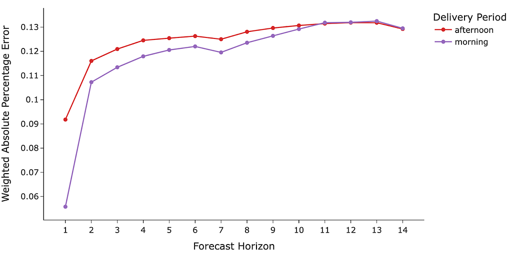
However the lack of formal testing, we do have strong evidence of the feature’s impact. Its effectiveness is strongly suggested by our current model’s performance. As shown in Figure 4, a visualization of the Weighted Absolute Percentage Error (WAPE or wMAPE) by forecast horizon highlights its exceptional short-horizon accuracy. Specifically, the prediction error for the 1-day ahead forecast decreases by an average of 20–50%.
We don’t want to fail to mention two things about this powerful feature. First, it sometimes feels like “cheating,” as we are including part of the target into the features at training time. Regardless, it worked pretty well (most of the time). Second, the feature has a great operational intuition that analysts trust, as they understand its meaning quite well and how it should impact the model. Currently, we have reduced the number of people required to check anomalous/missing forecasts to just one per market, which has allowed more analysts to focus on other initiatives.
In Figure 2, we saw a manual update of the initial forecast, based on deviations from confirmed deliveries rate. Below we show how our current TFT model reacts to the same deviations. The first update happens around 7 am, decreasing the predicted delivery count, as the current number of confirmed deliveries looks lower than the expected (the model learns the concept of what “a regular day” looks like during training.) After that, as the confirmed deliveries get closer and closer to the expected behavior, the forecast gets updated once again, this time upwards. After 10 am, as we are receiving more deliveries than expected, the forecast updates once again, this time for above the initial prediction, awesome! This behavior allowed us to ensure we provide our analysts and operational teams with an always up-to-date value.

Fundamental problems we found out
For quite some time, the confirmed deliveries feature felt like a silver bullet. It boosted short-term accuracy, planners trusted it, and it reduced manual corrections. But as our system matured and our expectations grew, cracks began to appear — not in the feature itself, but in the foundations it forced us to build around it.
Reconstructing the past, and the context about it
The first uncomfortable realization was that we had partially lost the ability to properly backtest our model. Confirmed deliveries are inherently stateful: their value depends on when you observe them. The number at 08:00 is different from the one at 10:00, and different again at 14:00. While we trained on five sampled moments per day, we had not historically stored a perfectly consistent snapshot of what the world looked like at each of those moments.
So whenever we wanted to answer a simple question — “what would the model have predicted last year at 09:00 for tomorrow’s deliveries?” — we had to reconstruct the past. That reconstruction was expensive, fragile, and sensitive to tracking changes over time. In practice, we were often validating the model on a partially synthetic view of history.
And confirmed deliveries never came alone. Intra-day forecasting forced us to also reconstruct the operational context of each moment: capacity changes and slot closures in particular. If a hub closed slots early, confirmed deliveries flattened — but that flattening reflected supply constraints, not necessarily lower demand. To teach the model the difference, we kept adding capacity-related features. Each iteration improved local behavior, but also increased system complexity. We had achieved a unified model — but at the cost of growing internal complexity.
Blur root causes, and persistent under-forecasting
As long as performance improved at short horizons, the trade-offs described above felt acceptable. But over time, another issue surfaced: it became harder to reason about failures.
Let’s imagine we started having problems with long-horizon forecasts. In a normal scenario where your model focuses only on day-level, the root cause should be relatively clear — seasonality shifts, market growth, calendar effects, etc. But in our case, with intra-day dynamics (i.e, the confirmed deliveries rate) tightly integrated into the same model, those boundaries blurred. Was a bad 7 days ahead forecast due to overfitting the confirmed deliveries rate? A misinterpreted capacity signal? Or simply holiday effects?
At the same time, one weakness remained stubborn: under-forecasting. Operationally, this is our most painful error. If we predict too few deliveries, capacity is not opened in time, vehicles and pickers are insufficient, and revenue is lost. Yet even after incorporating confirmed deliveries as an input, the model sometimes predicted fewer deliveries than were already booked.
So overall we found out 3 types of issues that were not easy to debug: (1) predicted deliveries below current confirmed deliveries, (2) severe under-forecasting after temporary capacity constraints (i.e., we had a problem but it solved, therefore the predicted demand should be similar as before having the issue), and (3) close to zero predictions (in practical terms model predicting zero demand).
Did we overfit the confirmed deliveries (rate)?
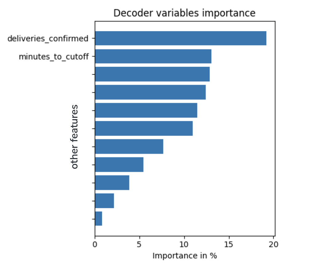
To investigate that possibility we looked into the feature importance of the model. In the case of a TFT, we need to look specifically at the multi-head self-attention decoder component, since it is the one in charge of using future and past encoded covariates to produce predictions. In our case, it looks like Figure 9 below. “Deliveries confirmed” is the most important feature with almost 20%, followed by “minutes to cutoff” at around 13%. These two features are the ones responsible for capturing the intra-day interpolation, surprise! (not really, we were suspecting this for a while.)
Fundamental conclusions we reached out
If there is something we learned through this journey, it is that a feature can be both your greatest ally and your most subtle trap.
Confirmed deliveries gave us exactly what we needed at a critical moment in our growth. It dramatically improved short-term accuracy, earned the trust of planners, and automated what used to be manual corrections.
But we hadn’t just added a feature — we had reshaped the system around it. Training data grew more complex, backtesting more fragile, and the model harder to reason about. We embedded operational logic — the interpolation between confirmed and final deliveries — deep inside a black box, trading transparency and control for performance.
Realizing we had to leave behind our best feature did not happen overnight. It emerged through strange backtests, stubborn under-forecasting, and long debugging sessions. But that discomfort gave us clarity. It forced us to confront the real architectural issues we had postponed for too long.
And that is where the story truly begins. In the next chapter, we’ll share how we redesigned the system to recover control, restore robustness, and keep the strengths of what worked — without letting a single feature dictate the future of the model.
Until then.
We are hiring! Check it out here:
Machine Learning Engineer | Engineering | Picnic Careers
The amazing journey of leaving behind your best feature was originally published in Picnic Engineering on Medium, where people are continuing the conversation by highlighting and responding to this story.


 Majid Hajiheidari